This post summarizes several methods in calculating distance-to-default (DD), which is an important factor in measuring a firm’s probability of default.

The Distance-to-Default

As the name suggests, distance-to-default (DD) measures how far a firm is away from default. Strictly speaking, the firm must have limited liability. DD has been widely used both in academic research and business applications. Moody’s EDF is one of the most famous applications that use DD to infer probability of default with an empirical mapping.

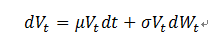
The definition of DD is based on Merton’s model, which assumes that firms are financed by equity and thus can be modeled as a call option on the underlying assets of the firm with a strike price equal to the book value of the firm’s liabilities. The asset value V follows a geometric Brownian motion.

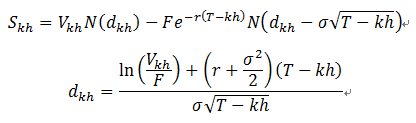
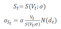
Then the equity value at time t by Black-Scholes option pricing formula becomes

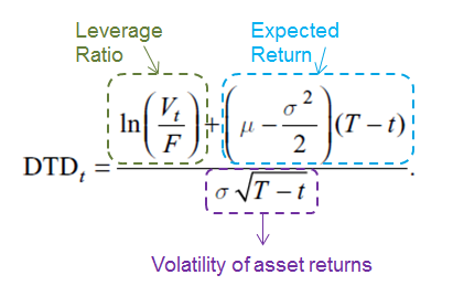
Then DD is defined as below. It can be seen as the logarithm of the leverage ratio shifted by the expected return and scaled by the volatility.

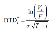
In practice, however, the asset return drift term cannot be estimated with reasonable precision using high frequency data over a time span of several years due to the nature of diffusion models. Therefore, DD is calculated in the following reduced form, which yields a more stable value. So in order to calculate DD, we need to first estimate asset drift and asset volatility.

The Market Value Proxy Method

Since the market value of asset is not directly observable and hard to determine, an intuitive alternative is to use the sum of equity value and the market value of liability. For public firms, it is easy to obtain the equity value, but the market value of liability is hard to estimate since most firms have a large portion of debt in some non-tradable forms. Therefore, the market value proxy method offers a hybrid approach of adding equity value to the book value of liabilities. Using the market value proxy method, it is straightforward to estimate the asset drift and asset volatility. However, it is argued that the market value proxy method provides an upward biased estimation of the asset value, which results in overestimation of DD.

The Volatility Restriction Method

By applying Ito’s lemma to both sides of the Black-Scholes option pricing formula, one can arrive at the following second equation decribing the relationship between asset volatility and equity volatility (the so-called volatility restriction).

Then together the two equations above have two unknowns, the asset value and asset volatility. So the two equation system can be solved at any given time point. In practice the volatility restriction method can be implemented through the following two approaches, which do not yield exactly the same results and thus create some inconsistency.

• Approach 1: solve the two-equation system repeatedly to get a time series of asset values, them compute the sample mean to obtain an estimate for 𝝁.
• Appraoch 2: solve the two-equation system once at a single time, and apply the obtained 𝝈 to all earlier time points to obtain a time series of implied asset values and then derive the 𝝁 from the time series.

The issue of the volatility restriction method is that the second equation linking equity and asset volatility holds only instantaneously. In practice the market leverage moves around far too much for the formula to provide reasonable results. It actually biases the probabilities in exactly the wrong direction.

The KMV Method

The KMV method improves on the volatility restriction method by replacing the second equation describing the volatility restriction with an iterative procedure consisting of the following steps:

• Step 1: Assign an initial value for asset volatility 𝝈.
• Step 2: Given asset volatility, use BSM equation to estimate a time series of asset values and hence corresponding asset returns.
• Step 3: Calculate the updated estimate for asset volatility from the implied asset returns obtained in step 2.
• Step 4: Repeat Step 2 and Step 3 until the convergence of asset volatility.

The following portion of code is an implementation of the KMV method in R.

  asset_value = timeSeries(rep(NA, length(equity_value)), time(equity_value))
  asset_volatility = equity_volatility  # initial estimate of volatility
  asset_volatility_old = 0
  index = 1
  while(abs(asset_volatility - asset_volatility_old)/asset_volatility_old > 0.0001) {  # iterative solution for asset values
    index = index + 1
    for(i in 1:length(equity_value)) {
      temp = uniroot(rooteqn, interval=c(equity_value[x], 1000*equity_value[x]), V=equity_value[x], rf=rf, sigma=asset_volatility, X=default_point, T=(T+1-(x-1)*h))
      asset_value[i] = temp$root
    }
    asset_volatility_old = asset_volatility
    asset_volatility = as.numeric(sd(weeklyReturn(asset_value, type = 'log'), na.rm = TRUE)) * sqrt(52)
  }

The Maximum Likelihood Estimation Method

The Maximum Likelihood Esimation (MLE) method here is assumed to be using the same definition of default point as the KMV method.

default point = short-term liabilities + 0.5 * long-term liabilities

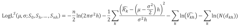
Then from assumption of Merton’s model that asset value follows a geometric Brownian motion, one can derive a log-normal distribution based of asset return. And the log-likelihood function of this log-normal joint distrubution can be transfromed from asset values to equity values. The detailed derivation is skipped here, but I do encourage you to derive this log-likelihood function below by yourself, which really helps in understadning the following discussions.

This log-likelihood function can be maximized by various optimization techniques, but here we are uisng the Expectation Maximization (EM) algorithm to solve this maximization problem. It can be shown later than this EM solution to the MLE method is the same as the KMV method both in theory and implementation. The EM algorithm is a natural generalization of maximum likelihood estimation to the incomplete data model, where in this case, the market value of asset cannot be observed (latent variables).

• Expectation step : evaluate the log-likelihood function conditioning the complete data (assign random initial guess for the unobserved).
• Maximization step: find new parameters that maximize the conditional expectation of log-likelihood function above.

In our case, the conditional expectation of log-likelihood function in E-step is

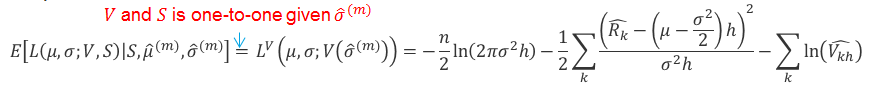
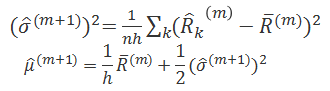
This is actually the original log-likelihood function of the asset values before transforming to equity values. And in M-step, maximizing the function above actually has the following analytical solution.

The following part of code is an implementation of the EM algorithm in R, where e_step and m_step are customized functions.

  for (it in 1:maxit) {
    
    if (it == 1) {
      ## initialization
      e.step <- e_step(asset_drift = 0, asset_volatility = equity_volatility, equity_value = equity_value, default_point = default_point, rf = rf, h = h , T = T, n = n)
      m.step <- m_step(e.step$loglik.func, e.step$asset_drift, e.step$asset_volatility)
      cur.loglik.value <- e.step$loglik.value
      loglik.vector <- cur.loglik.value
    } else {
      ## repeat E and M steps untill convergence
      e.step <- e_step(m.step$asset_drift, m.step$asset_volatility, equity_value = equity_value, default_point = default_point, rf = rf, h = h , T = T, n = n)
      m.step <- m_step(e.step$loglik.func, e.step$asset_drift, e.step$asset_volatility)
      new.loglik.value <- e.step$loglik.value
      loglik.vector <- c(loglik.vector, new.loglik.value)
      
      loglik.diff <- abs(cur.loglik.value - new.loglik.value)
      if(loglik.diff < 1e-6) {
        break
      } else {
        cur.loglik.value <- new.loglik.value
      }
    }
  }